Shapley Values and Regressions
Multicollinearity Approach with Shapley Values to Regressions
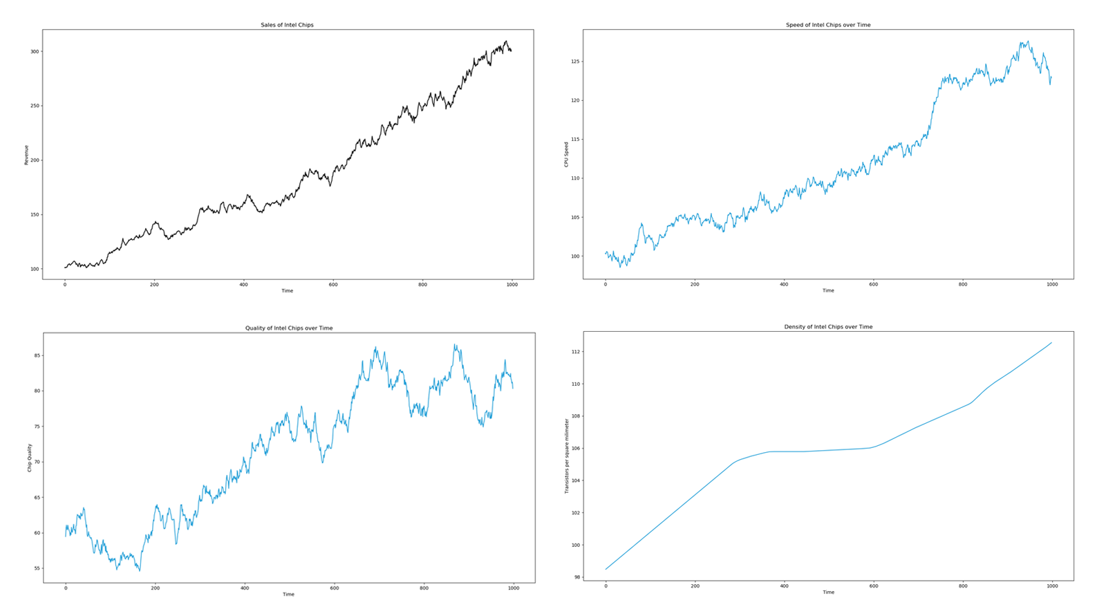
Lloyd Shapley was an American Mathematician who won the Nobel-Prize in economics. One of his greatest contributions was the concept of a Shapley value in the field of cooperative game theory. Recently, econometricians have adopted Shapley values as a way to tackle multicollinearity in regressions. It is a highly peculiar approach since one can view a regression as a game between multiple independent variables X competing to see who has the greatest impact on the dependent variable Y. Consider a simple regression with 3 independent variables: $$ Y=\alpha + \beta_1 X_1 + \beta_2 X_2 + \beta_3 X_3 + \epsilon$$ The approach utilized to dealing with muticollinearity with Shapley values involves running multiple permutations of regressions to see which factors truly have the strongest influence on Y and averaging out those contributions. In our three case scenario the total number of permutations of regressions we could run is equal to the factorial of the number of our independent variables X (6): $$ Y=\alpha + \beta_1 X_1 + \epsilon$$ $$ Y=\alpha + \beta_2 X_2 + \epsilon$$ $$ Y=\alpha + \beta_3 X_3 + \epsilon$$ $$ Y=\alpha + \beta_1 X_1 + \beta_2 X_2 + \epsilon$$ $$ Y=\alpha + \beta_1 X_1 + \beta_2 X_2 + \epsilon$$ $$ Y=\alpha + \beta_2 X_2 + \beta_3 X_3 + \epsilon$$ $$ Y=\alpha + \beta_1 X_1 + \beta_2 X_2 + \beta_2 X_3 + \epsilon$$ First we would check how much each independent variable X impacts the dependent variable Y. We then check how different combinations of two variables impact Y. At the end we can check how much of an impact they all have together. This gives us our R-squared values for all of the possible ways Y can be impacted. Now we utilize the Shapley formula which can be basically expressed for econometrics as: $$ \varphi (\beta_i )=\frac {1}{!X} \sum_{coalitions \; excluding \; beta_i}\frac{marginal \; contribution \; of \; \beta_i \; to \; coalition} {number \; of \; coalitions \; excluding \; \beta_i \; i} $$ This will give us the correct beta for each independent variable. Suppose we are a chip manufacturer like Intel and we are looking to adjust our budget to allocate capital across three segments which we think drive our revenue for chip sales. We think that chip speed, chip density, and chip quality are our main factors that impact our sales. We want to figure out how much we could allocate to each department in order to get the best bang for the buck in the future. We at first construct our regression as: $$ Y_{sales} =\alpha + \beta_{s} X_{s} + \beta_{d} X_{d} + \beta_{q} X_{q} + \epsilon$$ Where s=speed, d=density, q=quality. I've generated a randomized data set for these variables and made them all drift upwards. The black graph is the dependent sales variable while the blue are the independent variables.
The first thing we notice when we run this regression is multicollinearity. Our coefficients are all over the place. This doesn't help us much when we have to allocate our budget for what will drive sales.
       OLS Regression Results
==============================================================================
Dep. Variable:                  sales   R-squared:                       0.976
Model:                            OLS   Adj. R-squared:                  0.976
Method:                 Least Squares   F-statistic:                 1.351e+04
Date:                Sun, 23 Sep 2018   Prob (F-statistic):               0.00
Time:                        12:16:38   Log-Likelihood:                -3629.0
No. Observations:                 999   AIC:                             7266.
Df Residuals:                     995   BIC:                             7286.
Df Model:                           3
Covariance Type:            nonrobust
==============================================================================
                 coef    std err          t      P>|t|      [0.025      0.975]
------------------------------------------------------------------------------
Intercept   -868.3913     16.928    -51.300      0.000    -901.609    -835.173
speed          5.0703      0.098     51.703      0.000       4.878       5.263
quality        0.3679      0.063      5.883      0.000       0.245       0.491
density        4.3654      0.244     17.869      0.000       3.886       4.845
==============================================================================
Omnibus:                       11.081   Durbin-Watson:                   0.069
Prob(Omnibus):                  0.004   Jarque-Bera (JB):               11.151
Skew:                           0.256   Prob(JB):                      0.00379
Kurtosis:                       3.072   Cond. No.                     9.92e+03
==============================================================================

Warnings:
[1] Standard Errors assume that the covariance matrix of the errors is correctly specified.
[2] The condition number is large, 9.92e+03. This might indicate that there are
strong multicollinearity or other numerical problems.
Presence of multicollinearity
Instead of applying ridge or lasso regressions which usually involve certain parameters that one has to estimate/guess in order to adjust the weights of each beta coefficient to deal with multicollinearity, we rather apply the Shapley formula where no such parameters are necessary and wherein for the values we substitute the adjusted R-squared values for each of the possible regressions. We run all of our possible combinations of regressions which give us the following R-squared values: $$ R^2_{speed}= 0.965 $$ $$ R^2_{quality}= 0.743 $$ $$ R^2_{density}= 0.899 $$ $$ R^2_{speed, quality}= 0.968 $$ $$ R^2_{speed, density}= 0.975 $$ $$ R^2_{quality, density}= 0.912 $$ $$ R^2_{speed, quality, density}= 0.976 $$ We know that these regressions are spurious and colinear so we use the Shapley value formula on these R-squared outputs. Each dependent variable can be seen as competing for its relevance in a game where the game is who's the most relevant at guessing sales. We can check how relevant it is not just by how much it impacts the dependent variable by itself, but also as the sum of all of its marginal contributions when it is a part of a coalition with other dependent variables (part of a multiple regression). We apply the Shapley formula as follows:
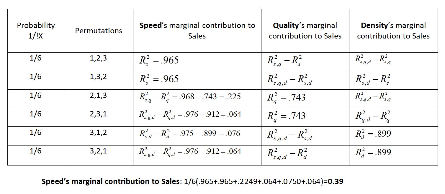
Showing with an example, we wind up getting a value of 0.39 for our Speed coefficient. Solving for all of the coefficients with Shapley we get: $$ \beta_{speed}= 0.39 $$ $$ \beta_{quality}= 0.25 $$ $$ \beta_{density}= 0.33 $$ These are our adjusted betas after being treated for multicollinearity. We can now use this information to help with our Intel capital budgeting decision by using the beta coefficients as our multipliers. If we have $100 million to allocate to next year's R&D budget, we'd allocate them as:
$$ $39,000,000 = speed $$ $$ $25,000,000 = quality $$ $$ $33,000,000 = density $$
Python Code for Multicollinearity Treatment with Shapley Values
Since doing the above calculation is an incredible nightmare, here is the code for applying Shapley values for multiple regressions. An interesting note to make is that the Shapley formula is factorial in its time complexity. This means that if you have 3 independent variables, then your Shapley calculation involves 6 regressions as was shown above in our Intel example. If you have 10 independent variable, then your Shapley calculation involves 3,628,800 regressions!
import numpy as np
import pandas as pd
import statsmodels.formula.api as sm
import shap

yd=pd.read_csv('sales.csv') # dependent variable data
xa=pd.read_csv('speed.csv') # independent variable 1
xb=pd.read_csv('quality.csv') # independent variable 2
xc=pd.read_csv('density.csv') # independent variable 3
yd=pd.DataFrame(yd)
xa=pd.DataFrame(xa)
xb=pd.DataFrame(xb)
xc=pd.DataFrame(xc)
series=pd.concat([yd,xa,xb,xc], axis=1)
series_unfiltered=pd.concat([yd,xa,xb,xc], axis=1)
series_unfiltered.columns=['sales','speed','quality','density']
series.columns=['sales','speed','quality','density']

result=sm.ols(formula='sales ~ speed + quality + density', data=series_unfiltered).fit()

print result.summary() # OLS shows us multicollinearity

def reg_m(y,x):
    ones=np.ones(len(x[0]))
    X=sm.add_constant(np.column_stack((x[0],ones)))
    for ele in x[1:]:
        X=sm.add_constant(np.column_stack((ele,X)))
    results=sm.OLS(y,X).fit()
    return results

regression_combos=shap.power_set(np.array(series.columns[1:]))

characteristic_fx={}

for i in xrange(0,len(regression_combos)):
    deps='+'.join(regression_combos[i])
    result=sm.ols(formula='sales ~ '+ deps, data=series_unfiltered).fit()
    print str(deps) + ' with R-squared of: '+ str(round(result.rsquared,3))
    characteristic_fx[str(','.join(regression_combos[i]))]= round(result.rsquared,5)

player_list = list(np.array(series.columns[1:]))

coalition_dictionary = characteristic_fx

g = shap.Coop_Game(player_list,coalition_dictionary)

print player_list # our list of independent variables
print coalition_dictionary # our list of all of the R-squared for all of the possible combinations
print 'Shapley adjusted beta coefficients are: ' + str(g.shapley())